Example 12: Source clustering power spectra
This sample script showcases the use of the NmtFieldCatalog class for source clustering.
import numpy as np
import healpy as hp
import matplotlib.pyplot as plt
import pymaster as nmt
import os
import wget
# This script showcases the use of catalog-based pseudo-C_ells
# in the case of a source clustering catalog.
# We start by initializing a lognormally distributed source density field at
# a given nside and a given source density and survey mask.
nside = 128
source_density = 0.001 # source number density per square arcmin
# We use as a basis the publicly available selection function for the
# Quaia sample.
fname_mask = 'selection_function_NSIDE64_G20.5_zsplit2bin0.fits'
if not os.path.isfile(fname_mask):
wget.download("https://zenodo.org/records/8098636/files/selection_function_NSIDE64_G20.5_zsplit2bin0.fits?download=1") # noqa
mask = hp.ud_grade(hp.read_map(fname_mask), nside_out=nside)
# Binarize it for simplicity
mask = (mask > 0.5).astype(float)
ls = np.arange(3*nside)
cl = 1./(ls + 10.)**2.
npix = hp.nside2npix(nside)
pix_area_arcmin = (4*np.pi/npix)*(180*60/np.pi)**2
deltaG = hp.synfast(cl, nside)
nmap_src = source_density*pix_area_arcmin*np.exp(deltaG
- 0.5*np.std(deltaG)**2)
# We then draw a Cox-distributed source catalog with lognormal intensity
# measure (i.e., a Poisson-sampled source catalog whose intensity is also
# stochastic).
num_src_mean = source_density * pix_area_arcmin
num_sources = int(np.amax(nmap_src*mask)*len(nmap_src))
# probability map for a random source to be sampled at a given pixel
pmap_src = mask*nmap_src/np.amax(mask*nmap_src)
def gen_poisson(pmap, nsrc):
cth = -1 + 2*np.random.rand(int(nsrc))
phi = 2*np.pi*np.random.rand(int(nsrc))
sth = np.sqrt(1 - cth**2)
unif = np.random.rand(nsrc)
vec = np.array([sth*np.cos(phi), sth*np.sin(phi), cth])
ipix = hp.vec2pix(nside, *vec)
good = unif <= pmap[ipix]
positions = np.array([np.arccos(cth[good]), phi[good]])
return positions
# draw random source positions with continous random angles
positions = gen_poisson(pmap_src, num_sources)
# We then draw Poisson-distributed random source catalog with 50 times higher
# number density than the source catalog.
nran_factor = 50
num_ran_mean = num_src_mean * nran_factor
nmap_ran = num_ran_mean * mask
pmap_ran = nmap_ran/np.amax(nmap_ran)
num_randoms = int(np.amax(nmap_ran)*len(nmap_ran))
positions_ran = gen_poisson(pmap_ran, num_randoms)
# We assign uniform weights to all sources and randoms.
weights = np.ones(len(positions[0])).astype(np.float64)
weights_rand = np.ones(len(positions_ran[0])).astype(np.float64)
# Now, we compute the mode coupling matrix at the positions and weights of the
# random catalog.
lmax = 3*nside-1
nmt_bin = nmt.NmtBin.from_lmax_linear(lmax, nlb=10)
lb = nmt_bin.get_effective_ells()
f = nmt.NmtFieldCatalogClustering(
positions, weights, positions_ran, weights_rand, 3*nside-1
)
wsp = nmt.NmtWorkspace.from_fields(f, f, nmt_bin)
# We compute the clustering field by passing both the source catalog and the
# random catalog.
pcl_uncorrected = hp.alm2cl(f.alm)
pcl = nmt.compute_coupled_cell(f, f)
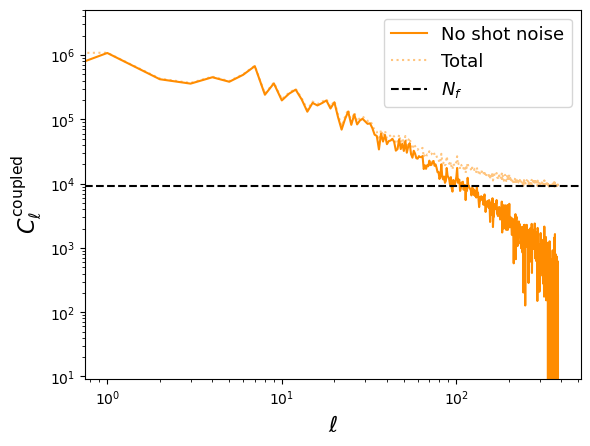
# We plot both the shot-noise corrected and uncorrected mode-coupled
# power spectrum.
plt.clf()
plt.plot(pcl.flatten(), label="No shot noise", color="darkorange", ls="-")
plt.plot(pcl_uncorrected.flatten(), color="darkorange", alpha=0.5, ls=":",
label="Total")
plt.loglog()
plt.xlabel(r"$\ell$", fontsize=16)
plt.ylabel(r"$C_\ell^{{\rm coupled}}$", fontsize=16)
plt.axhline(f.Nf, color="k", linestyle="--", label=r"$N_f$")
plt.ylim((f.Nf/1000, None))
plt.legend(fontsize=13)
plt.savefig("sample_clusteringcatalog_coupled.png", bbox_inches="tight")
plt.show()
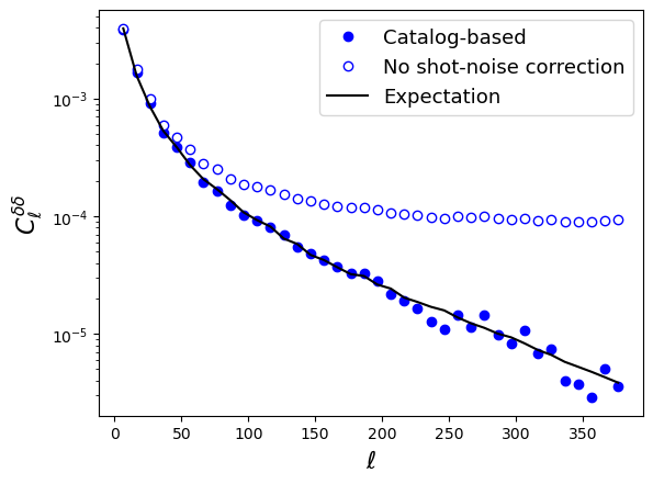
# Now, we compute the decoupled overdensity power spectrum
clb = wsp.decouple_cell(pcl).squeeze()
clb_uncorrected = wsp.decouple_cell(pcl_uncorrected).squeeze()
# Finally, we compute the binned theory power spectrum and compare with data.
# Because of the lognormal transformation, this is different from the
# theoretical power spectrum we started with, so we just compute it from
# the mean density map before Poisson sampling and masking.
delta = nmap_src/np.mean(nmap_src) - 1
clt = hp.anafast(delta)
# We annoyingly need to divide the pseudo-C_ell by the pixel window function
# imprinted on the source field values by the (pixelized) density map. Since
# the real sky does not have a pixel window function, you wouldn't need to
# do this for real data!
clt = (clt*hp.pixwin(nside)**2)[:lmax+1]
pcl_clean = wsp.couple_cell(clt.reshape((1, -1)))
cl_clean = wsp.decouple_cell(pcl_clean).flatten()
plt.clf()
plt.plot(lb, clb, "bo", label="Catalog-based")
plt.plot(lb, clb_uncorrected, "bo", mfc="w", label="No shot-noise correction")
plt.plot(lb, cl_clean, "k-", label="Expectation")
plt.yscale('log')
plt.legend(fontsize=13)
plt.xlabel(r"$\ell$", fontsize=16)
plt.ylabel(r"$C_\ell^{\delta\delta}$", fontsize=16)
plt.savefig("sample_clusteringcatalog_decoupled.png", bbox_inches="tight")
plt.show()
The result of running this is: