Example 11: Catalog-based power spectra for spin-s fields

This sample script showcases the use of the NmtFieldCatalog class for spin-2 source catalogs.

import numpy as np
import healpy as hp
import matplotlib.pyplot as plt
import pymaster as nmt
import wget
import os


# This script showcases the use of catalog-based pseudo-C_ell
# in the case of a masked spin-2 field catalog.

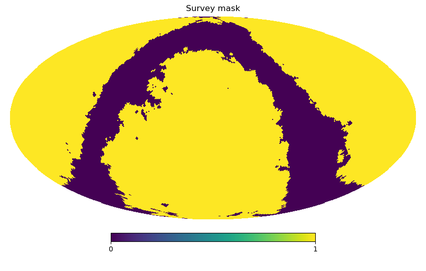
# We start by creating a pixel-level survey mask
nside = 128
# We use as a basis the publicly available selection function for the
# Quaia sample.
fname_mask = 'selection_function_NSIDE64_G20.5_zsplit2bin0.fits'
if not os.path.isfile(fname_mask):
    wget.download("https://zenodo.org/records/8098636/files/selection_function_NSIDE64_G20.5_zsplit2bin0.fits?download=1")  # noqa
mask = hp.ud_grade(hp.read_map(fname_mask), nside_out=nside)
# Binarize it for simplicity
mask = (mask > 0.5).astype(float)
hp.mollview(mask, title="Survey mask")
plt.savefig("sample_shearcatalog_mask.png")
plt.tight_layout()
plt.show()

# We then draw 1e7 random sources uniformly distributed across the masked sky
num_sources = 1e7
cth = -1 + 2*np.random.rand(int(num_sources))
phi = 2*np.pi*np.random.rand(int(num_sources))
sth = np.sqrt(1 - cth**2)
angles = np.array([sth*np.cos(phi), sth*np.sin(phi), cth])
ipix = hp.vec2pix(nside, *angles)
good = mask[ipix] > 0
# theta, phi
positions = np.array([np.arccos(cth[good]), phi[good]])

# For simplicity, these sources have uniform weights.
weights = np.ones_like(positions[0])

# Then, we generate a Gaussian spin-2 field with only E-modes, to mimic e.g. a
# cosmic shear field.
ls = np.arange(3*nside)
cl = 1./(ls + 10.)**2.
cl0 = 0*cl
map_Q, map_U = hp.synfast([cl0, cl, cl0, cl0], nside, new=True)[1:]
catalog_Q = map_Q[ipix][good]
catalog_U = map_U[ipix][good]

# Now, we compute the mode coupling matrix of the source catalog.
lmax = 3*nside-1
nmt_bin = nmt.NmtBin.from_lmax_linear(lmax, nlb=10)
lb = nmt_bin.get_effective_ells()
# Note that we pass `None` as the field value, since we
# will only use `f` to compute the mode-coupling matrix.
f = nmt.NmtFieldCatalog(positions, weights, None, lmax=lmax,
                        lmax_mask=lmax, spin=2,
                        beam=hp.pixwin(nside, lmax=lmax))

# Note also that we assigned a "beam" to this field corresponding
# to the pixel window function of the maps used to create the
# field value of each catalog source. Since the real sky does
# not have a window function, this should in general not be
# necessary!

wsp = nmt.NmtWorkspace.from_fields(f, f, nmt_bin)

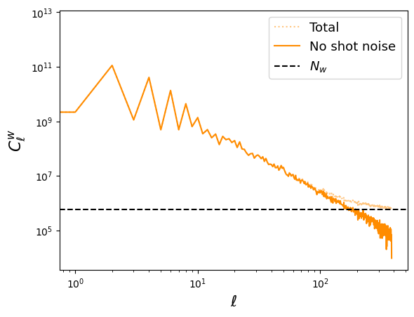
# We compute and plot the survey mask's pseudo power spectrum, highlighting
# the contribution of the mask shot noise.
pcl_mask = hp.alm2cl(f.get_mask_alms())
plt.clf()
plt.plot(pcl_mask, color="darkorange", alpha=0.5, ls=":", label="Total")
plt.plot(pcl_mask - f.Nw, label="No shot noise", color="darkorange", ls="-")
plt.loglog()
plt.axhline(f.Nw, color="k", linestyle="--", label=r"$N_w$")
plt.ylabel(r"$C_\ell^w$", fontsize=16)
plt.xlabel(r"$\ell$", fontsize=16)
plt.legend(fontsize=13)
plt.savefig("sample_shearcatalog_mask_pcl.png", bbox_inches="tight")
plt.show()

# We then compute the coupled spin-2 pseudo power spectrum
f = nmt.NmtFieldCatalog(positions, weights, [catalog_Q, catalog_U],
                        lmax=lmax, lmax_mask=lmax, spin=2,
                        beam=hp.pixwin(nside, lmax=lmax))
pcl = nmt.compute_coupled_cell(f, f)

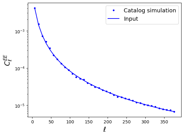
# Finally, we compute the decoupled power spectra, the binned theory
# expectation, and plot them.
clb = wsp.decouple_cell(pcl)
clb_theory = wsp.decouple_cell(wsp.couple_cell([cl, cl0, cl0, cl0]))

plt.clf()
plt.plot(lb, clb[0], "b.", label="Catalog simulation")
plt.plot(lb, clb_theory[0], "b-", label="Input")
plt.yscale('log')
plt.ylabel(r"$C^{EE}_\ell$", fontsize=16)
plt.xlabel(r"$\ell$", fontsize=16)
plt.legend(fontsize=13)
plt.savefig("sample_shearcatalog_decoupled.png", bbox_inches="tight")
plt.show()

The result of running this is: